Reinforcement Learning II: Decision Theory | Introducing Markov Decision Processes

Hello and welcome to this series on reinforcement learning! In this post we will discover what markov decision processes (MDP) are as well as what the markov property and markov chains are and how they all relate to each other. We will learn what a state transition probability matrix is and what a reward function is.

Understanding MDPs is very important as they lie at the foundation of almost all reinforcement learning. Algorithms that solve reinforcement learning problems actually solve variants of MDP. Thus by understanding what MDPs are you are much better poised to understand the algorithms that solve them.

I hope you are eager to read this post and to learn about MDPs! Make sure to treat yourself to a nice brew of coffee and some snack to keep the energy levels up as this post might be a bit intensive. Ready? Good. Welcome to the learning journey, and let’s go!

Wikipedia Definition of MDPs

When learning about reinforcement learning it is inevitable to learn about markov decision processes. A MDP is a framework to think about specific environments or problems where the outcomes are somewhat uncertain, but where we have choices that can affect the probabilities of different outcomes. I.e. there is an stochastic element to the problem (Stochastic means random).

Wikipedia defines and explains the Markov Decision Process as follows below. If at first it doesn’t make much sense to you the first time you read it – don’t worry. We will go through every bit of it and by the end of this article it will all make complete sense. :)) What they call process we call environment, and the decision maker is the agent.

Definition:

“At each time step, the process is in some state s, and the decision maker may choose any action a that is available in state s. The process responds at the next time step by randomly moving into a new state s’ and giving the decision maker a corresponding reward R_a(s,s’).

The probability that the process moves into its new state s’ is influenced by the chosen action. Specifically, it is given by the state transition function P_a(s,s’). Thus, the next state s’ depends on the current state s and the decision maker’s action a. But given s and a, it is conditionally independent of all previous states and actions; in other words, the state transitions of an MDP satisfies the Markov property.

Markov decision processes are an extension of Markov chains; the difference is the addition of actions (allowing choice) and rewards (giving motivation). Conversely, if only one action exists for each state (e.g. “wait”) and all rewards are the same (e.g. “zero”), a Markov decision process reduces to a Markov chain. “

So, the definition says that we have an environment (the process) with specific states in which the agent (the decision maker) can act with actions. These actions can lead to new states and can give rise to rewards. This should all be familiar to if you read the previous article (which you definitely should read before this one).

New concepts are the markov property and the markov chains terms. These will be made clear below.

Markov Property

Let’s start with the markov property.

A stochastic (random) process has the markov property if the conditional probability distribution of future events ONLY depends on the present state, and not on the sequence of events that lead up to it. The conditional probability distribution p(y|x) means “what is the chance of y, given x?”. As an example we might want to know what the probability of me being wet is given that it rains and that I’m outside, expressed as p(am_wet|rains, am_outside).

Wikipedia gives a good example with urns in explaining the markov property. I’ll reiterate it here. Let’s say that you have a urn with three balls in it – one red, one yellow and one black ball. The game (process) is to draw a ball for two time steps and then guess what colour the third ball will be. We will play this game in two variants. The first variant is where we draw a ball each time step and puts it to the side. This is called “without replacement”. The second variant is where we draw a ball each time step and then puts it back in the urn at the end of the next turn. As will be shown, the markov property holds for the second variant but not the first.

We begin playing the first variant of the game (without replacement). We put our hand in the urn and blindly chooses one ball. It’s the black ball. This puts us in the state of drew_black. We put the ball to the side, and the urn now contains only the red and yellow balls. Next time step we draw a red ball. This means that our next state is drew_red. We put the red ball to the side and the urn contains only the yellow ball. We now want to know the conditional probability of drawing the yellow ball.

This is rather easy given that we know what we drew in both our current and previous state. We know there are only one ball each of the colour red, black and yellow. If we know that we drew the red now and before that drew the black ball, our conditional probability of drawing the yellow ball is 1, meaning a 100% chance. We call this conditional probability p_h, where h stands for history. If we only knew our present state however, the conditional probability p_p would be 1/2, since the ball then could be either black or yellow (if we only know that we drew a red this time step).

p_h(yellow|drew_black, drew_red) = 1

p_p(yellow|drew_red) = 1/2

In this variant of the game not only the current but also the past informs the future. As we can see the conditional probability p_h is different from p_p. Thus the markov property does not hold for this game.

In the second variant of the game however, we put the ball back at each time step after drawing it (with replacement). We start the game with the urn containing a black, a red and a yellow ball. The first time step we draw the black ball. This puts us in the state drew_black. The urn now contains the red and yellow ball since we’re still in the first time step and only puts the ball back at the end of the next time step.

We then go to the second time step and draw the red ball. This puts us in the state drew_red, and we finish the turn by putting back the black ball from the previous turn. The urn now contains the black and the yellow ball. Now, what is the conditional probability of us drawing a yellow ball next time step? We know that our current state is drew_red, which means that the urn contains a black and a yellow ball. Thus the conditional probability p_p of drawing a yellow ball given we just drew a red ball is 1/2. Incorporating the previous state, drew_black, gives us no additional information, since p_h also is 1/2. We can in other words fully compute the conditional probability of the future states given only the present knowledge. Thus the markov property holds for this second example.

p_h(yellow|drew_black, drew_red) = 1/2

p_p(yellow|drew_red) = 1/2

Markov Chains and State Transitional Probabilities

Consider the following scenario: Let’s imagine that we have a very simple process with the three states A, B and C. If we are in state A we go to state B with 100% probability. If we are in state B we go to state C with 100% probability and likewise if we are in state C we go to state A with 100% probability. This very simple process can be illustrated by the image below:

In the above image the process is represented as a probabilistic graph. The states are represented by the red circles, and the arrows show where we can go in the next time step. So from A there is an arrow to B, meaning we can from A go to B. The number represents the probability of taking that route. In this case the probability of going to the next state is 1, meaning we always go to the next state. Upon further inspection of the process we can clearly see that this game holds true for the markov property: we can fully know the probabilities of the next state given our current state.

This game is what we call a markov chain. It is a process with defined states and where we randomly go to the next state based on some probability. The process also needs to obey the markov property discussed above in order to be a markov chain.

Before we go on to more interesting processes we need to introduce the transition probability matrix T. In this matrix each row i will represent the state we are in, and each column j will represent the states we can go to. The element (i,j) thus represents the probability of going from state i to state j. For our process above the state transition matrix would look as follows:

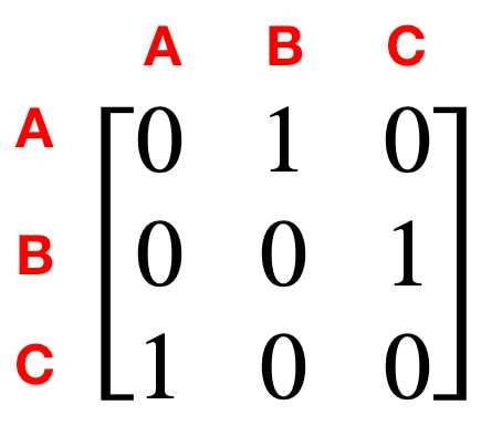
So if we want to know if we can go from B to A we can just look up T[1,0] = 0, and know that there is no chance of going directly from B to A.

A Slightly More Complex Markov Chain

Now this first example served nicely as an introduction onto more complex markov chains. Let’s look at a slightly more complex example, where the process above is expanded by the introduction of an arrow going from C to B with .5 probability. This would look as follows in graph form and yield the following state transition matrix:

The total chance for every row still adds up to 1, where the probability is equally split between A and B for row C. Let’s look at one more example, this time a bit more complicated.

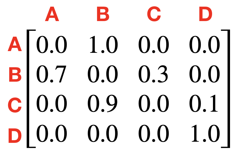
Okay, so let’s pause and look at what just happened. In this graph, A goes to B always, and B goes either to A or C. From C we go to B in most cases but with a small chance, 0.1, we go to D instead. And D has an arrow going to itself. This means that from D we go to D in the next time step. Ergo, once we hit D we stay in D for all future. This is called a terminal state and is a very important concept in markov chains and markov decision processes. Terminal states are end states.

Let’s briefly return to the concept of conditional probability and the markov property. Given that the current state is B, what is the probability that the next state will be A? Well, just by looking at either the graph or the matrix we can see that p(A|B) = 0.7. Likewise we can tell that p(C|B) = 0.3 and p(C|A) = 0 (as there is no arrow going from A to C). We also clearly see that no information about previous states are needed as the next state is solely dependent on the current state. Thus, we can feel assured that the markov property holds for our process and that it is a markov chain.

We now know all that we need to know in order to understand the Markov Decision Process. So let’s begin…

Markov Decision Processes

In a markov chain, the next state is randomly selected conditioned on the current state. With the markov decision process however this model is expanded to include the choice of actions and also to include the notion of reward for being in certain states. The rewards means that some states can be more preferable to be in than other states. The actions means that we can affect our state by what actions we take. However, the process is still stochastic as the outcome of actions might be uncertain.

In order to understand what’s new in an MDP, let’s work with a really simple example. Let’s say that our process is a game that consists of throwing a single die until you get a six. If the die shows a six you get 1 point, any other number you get the option to throw again or to quit. Each time you throw the die but it does not show a six it costs you 0.1 points. If you choose to quit the game you to lose 0.5 points. This game drawn as a graph looks as follows:

So in the graph we have the 3 states A, B and C. A represents us playing the game but not having won yet. When in state A we can either take the action A0 called “throw die” or the action A1 called “quit”. The actions are represented by the red arrows. If we take action A0 there is 1/6 chance that we get a six and win, and a 5/6 chance we don’t get a six and have to play again. Note that both C and B are terminal states. Previously we illustrated terminal states with an arrow looping from the terminal state to itself but here that arrow is omitted. This is to show that both ways of illustrating a process is valid and you will encounter both types of illustrating. The technical difference between having a loop or not in terminal states is whether the game is infinite or finite. But let’s not get ahead of ourself!

Don’t be scared! It might look intimidating but it really isn’t!

From the graph we can create the two reward matrices, R_throw and R_quit, as well as the two transition probability matrices P_throw and P_quit.

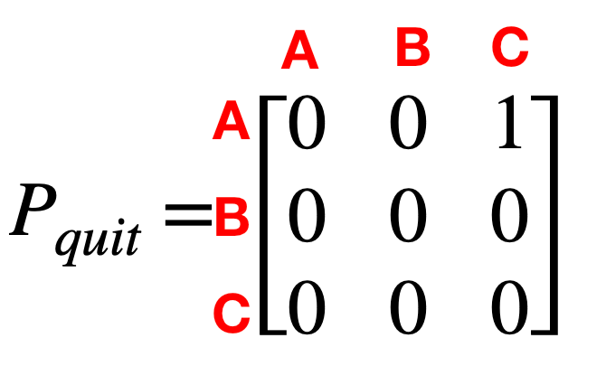
The reward matrices show the rewards for going from one state to the other and the transition probability matrices are the same as for the markov chain, except we now have one matrix for each possible action instead of a single one for the whole process. You should really go through each matrix and make sure you understand why it has a zero or other value in each place and how it relates to the graph. Start with P_quit. The only way for you to actually learn this is to do the hard work of making sure you understand how something is made in order to be able to recreate it. Just glancing briefly at the matrices won’t cut it. So go through them now.

Done going through the matrices? Good.

This case is very similar to the markov chain examples shown before. Our agent is still in one of several possible states. In each state there are transition probabilities to other states. The difference is that we in the MDP are given the option of what actions to take. We can imagine choosing between actions as choosing which transition probabilities we want to use. The outcome is still random, but at least we have some power to choose which odds we want to play.

And that is basically what a markov decision process is. It is a problem of optimal control where we are given some environment with different states and actions with unknown outcome. The “game” or the problem to solve is to find the optimal set of actions conditioned on the current state, that leads us to the greatest probability of the highest expected total reward. For our game of dice the decision would be whether to play the game or to quit, and for how long to play the game until we quit.

A Slightly More Complex MDP

Okay, so our next example will be slightly more involved but still manageable. This process simulates an agent who is lost in a forest and who wants to get home as fast as possible. The problem is that the forest is filled with traps in the form of deep pits. Every time the agent moves he risks falling into one of the traps. Luckily, if the agent falls into a trap he can attempt to escape by climbing up the sides of the trap. But this is not guaranteed to succeed and the agent risks falling back down into the trap – causing him to loose more time. The agent can choose to either walk slowly or to run fast as he tries to get home. If he runs he can cover more ground and is thus likelier to find his way back faster. But he is also more likely to fall into a trap as he is less careful. The decision problem is whether to walk or to run. The full probabilities are shown in the graph below.

For this MDP we have the set of states S = [Forest, Trapped, Home] and the state of actions A = [walk, run, escape]. The reward matrices R and transition matrices P for this process are as follows:

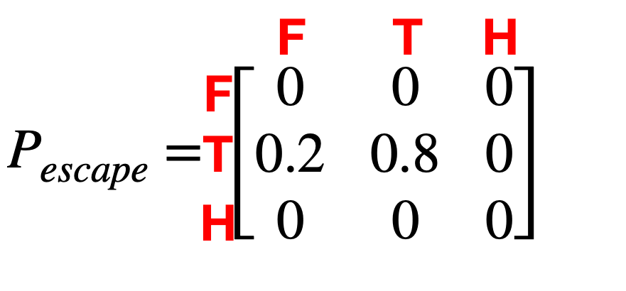
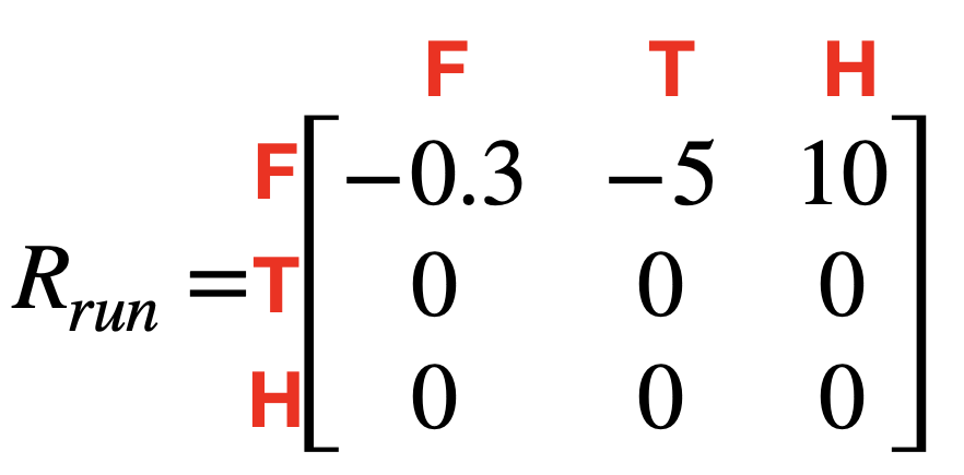
Again, if you feel overwhelmed take a sip of your coffee and breathe. Break it down by taking the first matrix P_run. Look at it and compare it to the graph. F is the forest. If we are in the Forest state and take the action run, what are the three arrows going out from it? Look back at the matrix. See? Additionally, looking at the states Trapped and Home we have no option of running and so the probabilities of getting to the next state by running if in any of those states is 0. Now go through the other matrices.

Looking Back At The Definition

Great job! You made it to the finish!

So we have now gone through the elements of the markov decision process. Let’s look back at the MDP definition from the begining of the post and see if our understanding has improved. To our aid we will look at it through the lens of the forest MDP example from above.

Definition of a Markov Decision Process:

“At each time step, the process is in some state s, and the decision maker may choose any action a that is available in state s. The process responds at the next time step by randomly moving into a new state s’ and giving the decision maker a corresponding reward R_a(s,s’).”

For our problem with the agent and the forest, we could be in the state s = “Forest” and choose action a = “Walk”. The process would then move into the new state s’ = “Trapped” with the probability 0.15 – given by looking up P_walk(Forest,Trapped). The reward R_a(s,s’) would be R_walk(Forest,Trapped) = -5.

“The probability that the process moves into its new state s’ is influenced by the chosen action. Specifically, it is given by the state transition function P_a(s,s’). Thus, the next state s’ depends on the current state s and the decision maker’s action a. But given s and a, it is conditionally independent of all previous states and actions; in other words, the state transitions of an MDP satisfies the Markov property. “

We saw this as the probability of both finding our way home and falling into a trap was higher if we ran than if we walked. And as we’ve already discussed the conditional probability p(s’|s,a) is only dependent on the current state and action and not any previous actions or states. And we already know what the markov property is.

“Markov decision processes are an extension of Markov chains; the difference is the addition of actions (allowing choice) and rewards (giving motivation). Conversely, if only one action exists for each state (e.g. “wait”) and all rewards are the same (e.g. “zero”), a Markov decision process reduces to a Markov chain. “

We already discussed how the markov decision process is an extension of the markov chain. By choosing actions we choose which transition probabilities we want to use, and we want to maximise our long term chances of getting the states with high rewards. But if a markov decision process has only a single action for each state there wouldn’t really be any choice and thus no decision to make as we only have a single transition matrix (since we only have a single action to take). A markov decision process with a single action and no rewards are thus simply a markov chain.

Closing Remarks

In this post we saw the definition of a MDP, we saw some examples of both markov chains and markov decision processes as well as we explored how to construct the reward matrix and the transition probability matrix. MDPs are a very powerful framework and can be used to model and reason about a host of problems as we will see in future posts.

In the next post we will explore how to solve MDPs in order to maximise the outcome in terms of rewards. Until then, have a good one and stay hungry for knowledge!