Hello and welcome to this post on how the K-Means Clustering algorithm works! In this post we will talk briefly about what clustering is. We will then proceed to gain some intuition for how the algorithm works before finally diving into a python code implementation of it. As always before we go into the details, make sure to grab a nice, fresh brew of coffe and a good snack for the energy levels. Ready? Great, let’s get to it and welcome to the learning journey!
What’s The Point of Clustering?
Clustering algorithms are useful when trying to find groups of similar data points in a given data set. For example if our data set is a bunch of fruits, a good clustering algorithms would ideally find that some fruits are more similar than others.
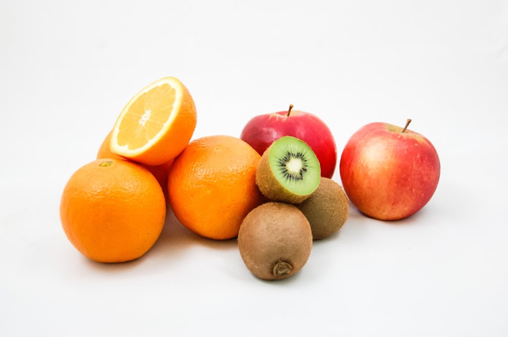
Let’s say that our data set is visualised by the image above. We could imagine that if we want to find out what groups can be found in this data set, a good clustering algorithm would return three groups; one containing the apples, one containing the kiwis and one containing the oranges. However, what constitutes the correct grouping might not always be so clear cut and we might sometimes want to do some other clustering.
For example, in the image above we can observe another possible clustering: fruits that are whole and fruits that are cut in half. Following that intention, a good clustering algorithm should return two groups. Or should we have six groups, with uncut oranges in one, cut oranges in a second, uncut kiwis in a third etc.? What is the correct answer?
Well, naturally the correct answer depends on what was your question. As is quite often the case in science – asking the correct question is half the answer. But let’s say that we have a data set and we know that we want to find k number of clusters – what would be a good way to divide the data points into k different groups? Well, there are many many different clustering algorithms each with it’s own set of advantages and disadvantages. In this post we will explore one of the most famous and easiest-to-understand algorithms: k-means clustering. But, before we delve into the mechanisms of k-means clustering we must first understand how we measure distance between data points.
Measuring Distances Between Points
The k-means clustering algorithm builds around finding k clusters in a data set. The algorithm defines a clusters of data points as points being “close” to each other. How close two points are to each other is defined by their distance.
There are several ways to define the distance between points, but the most common is the Euclidean distance. This is the distance you would get if you took a ruler and measured the straight path between two points. A nice property of this Euclidean distance is that it also is easy to generalize to any number of dimensions – i.e. we are not limited to only 1, 2 or 3 dimensions!
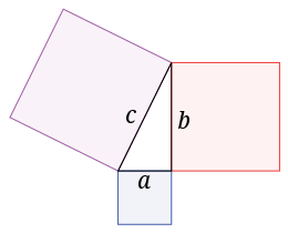
The Euclidean distance is built around the Pythagorean theorem. Let’s consider a right triangle with the hypotenuse c (the longest side of the triangle) and the two other sides a and b. The theorem states that the equation c2 = a2 + b2 holds for all right triangles. Thus, the length c can be rewritten as c = sqrt(a2 + b2), where sqrt() is the square root function.
From this Pythagorean theorem we can now derive our distance function. Let’s imagine that we have two points A and B in 2D-space. The distance between these two points can be easily calculated if we imagine them being two corners of a right triangle (and neither being in the right corner). The distance between A and B is then simply the hypotenuse c of this triangle. The length a and length b is the distance between the two points in the x-axis and y-axis, respectively.
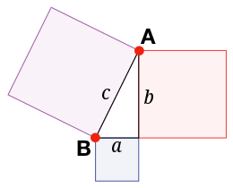
To take an easy example, let’s say that A=(3,4) and B=(5,1). The distance in the first dimension is then a = 3-5 = -2 and the distance in the second dimension is b = 4-1 = 3. Thus, we can easily compute the hypotenuse c with the Pythagorean theorem:

In three dimensions with A = (3,4,2) and B = (5,1,1) we just add the last dimensions as:

In fact, we can extend this to any dimensions. Thus, we can compare the distance between any two n-dimensional data points A = (a1, a2, … , an) and B = (b1, b2, …, bn) as:

Implementing this distance function in code is very easy.
def dist(A,B):
    d = 0
    for i in range(len(A)):
        d += (A[i]-B[i])**2
    return d**0.5
The method dist takes two vectors A and B as arguments. We then initialise a variable d to 0, which will be our distance. Then, we add the squared difference (ai-bi)2 between for every element i in the two vectors. We then take the square root of d and return it.
K-Means Clustering | Intuition
Now, armed the knowledge of how to measure the distance between two data points we are ready to dive into the algorithm itself.
The K-Means Clustering algorithm works by making an initial (random) assumption of the centers of k clusters. Once the centers are initialised, the algorithm goes through each point in the data set and looks at which center is the closest. The data point is then set to belong to the cluster corresponding to that center. The algorithm goes through all the data points and classifies each data point as belonging to one of the centers / clusters. Once this is done the clustering has been updated. The algorithm then computes a new center for the cluster, and the process repeats for this new center. Once no cluster changes it’s center or equivalentely once no data point switches cluster, the algorithm finishes and the clustering is done.
This is pretty abstract without any visualisations, so I’ve made a GIF below to illustrate the process.
As the parameter k is given by the user, the k-means algorithm requires us to decide how many clusters we want to use. There are methods of deciding the optimal number of clusters automatically, but we will not go into those in this post. Below is the same data set clustered by the k-means algorithm using four different values for k. The values for k are 2, 3, 4 and 5 respectively.

So again, the algorithm makes an initial random (blind) guess as to where the center of a cluster is. Then each point is classified according to the closest cluster center point. The centers are recomputed as the mean of the data points belonging to it’s cluster, and the process is repeated. Once the algorithm has converged and no updates are made to the clusters the algorithm is finished.
Let’s look at how this algorithm can be implemented in code!
K-Means Clustering | Python Implementation
We start by importing some libraries we will use:
from numpy.random import rand, randint
from sklearn.cluster import k_means
import numpy as np
import seaborn as sns
import pandas as pd
import matplotlib.pyplot as plt
We then proceed to generate some random 2D data points we want to cluster.
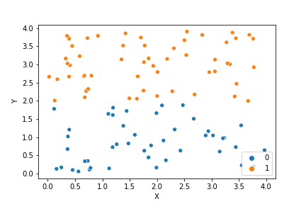
data = np.array([rand(2)*4 for i in range(100)])If we plot this data it looks like this:
Input: plt.scatter(data[:,0],data[:,1])

Output:
method: distances()
In order to write our code we will have to write some subroutines first. We will start with the method for measuring distances, which we’ll convieniently call distances(). The distances method will take as input two variables: point which is the data point and centers which are the centers of the clusters from which we want to measure the distance.
With our data produced above and k = 2, these variables can look as follows:
Input: print(point)

Output: array([1.49864859, 0.26361095])

Input: print(centers)

Output:
array([[2.27786443, 1.95684099],
       [0.25852261, 1.26453851]])

Input: distances(point,centers)

Output: array([1.86392202, 1.5936651 ])
So, point has x-coordinate 1.49 and y-coordinate 0.26. The two centers are positioned at the coordinates (2.27, 1.97) and (0.26, 1.26). The distances between the point and these two centers are 1.86 and 1.59 respectively. Thus, the point is closest to the second center and will be classified as belonging to the second cluster.
Implemented in code the distances method looks like:
def distances(point,centers):
        def dist(A,B):
            d = 0
            for i in range(len(A)):
                d += (A[i]-B[i])**2
            return d**0.5
        d = np.zeros(len(centers))
        for i,center in enumerate(centers):
            d[i] = dist(point,center)
        return d
method: intialise_centers()
The next method we will write is initialise_centers(), a method used to initialise the center points. There are many ways in which this could be done. For this example we will choose a very simple version where the method randomly selects two data points and finds the mean value of the two. This is done once for each of the k clusters.
def initialise_centers(data,k):
    N = len(data)
    centers = []

    for i in range(k):
        two_random_points = [data[randint(0,N-1)],
                             data[randint(0,N-1)]]
        center = np.mean(two_random_points,axis=0)

        while(str(center) in str(centers)):
            two_random_points = [data[randint(0,N-1)],
                                 data[randint(0,N-1)]]
            center = np.mean(two_random_points,axis=0)
        centers.append(center)
    return np.array(centers)
The method starts by initiating an empty list called centers. The method then goes through each of the k clusters and selects two random points from the data set. Next the method computes the center as the mean value of these two random points. As the points are randomly chosen, we also need to check that this center point isn’t already occupied as the center of another cluster (as that would break the algorithm). This is done with a while-loop.
method: update_clusters()
The next method is the update_clusters() method. This method takes the data and the centers as input. From this, the method recomputes the closest center for each data point and updates the cluster that data point belongs to.
def update_clusters(data,centers):
        new_clusters = []
        for point in data:
            d = distances(point,centers)
            new_clusters.append(np.argmin(d))
        return np.array(new_clusters)
method: update_centers()
The final method is the update_centers() method. This method takes as input the data, the clusters and the parameter k. The method then computes the new centers from the clustering of the data. This is done using the numpy mean method. The method iterates over all the clusters in a for loop, and selects all the data points that belong to that cluster, using the data[clusters==i] code. The new center points are then returned.
def update_centers(data,clusters,k):
    new_centers = [np.zeros_like(data[0]) for i in range(k)]
    for i in range(k):
        new_centers[i] = np.mean(data[clusters==i],axis=0)
    return np.array(new_centers)
method: kmeans()
We are now finally ready to put it all together. We begin by defining the method kmeans(), which will take as input the data and the parameter k, which decides how many clusters we want to find.
We start by initialising the centers and the clusters. We then create the variable centers_updated which will keep track of whether the centers has changed position. When the centers don’t change, i.e. when the update_centers() returns the same centers as we already had. This variable will be used as the condition in a while loop, which will run as long as the centers have not converged.
In the while loop we copy the centers in a temporary variable called old_centers. We then update the centers and then update the clusters (important that it is in that exact order!). Finally, we will update our boolean variable. This is done by summing the differences between centers and old_centers, and if the difference between the two is larger than 0 it means the centers have updated and the boolean will be true.
def kmeans(data, k = 3):

    centers = initialise_centers(data,k)
    clusters = update_clusters(data,centers)
    centers_updated = True

    while(centers_updated):
        old_centers = centers.copy()
        centers  = update_centers(data,clusters,k)
        clusters = update_clusters(data,centers)
        centers_updated = np.sum(np.abs(centers-old_centers)) > 0

    return clusters
bonus method: draw_clusters()
As a nice extra we can create the draw_clusters() method to visualise the data and the corresponding clustering. This will be done using the pandas library and looks as follows:
def draw_clusters(data,clusters):
    pdata = pd.DataFrame(data,columns=["X","Y"])
    f,ax = plt.subplots(1)
    sns.scatterplot(x="X",y="Y",hue=clusters,data=pdata)
    plt.show()
K-Means Clsutering | The Code Put Together and Evaluated
The code in it’s entirety looks as follows:
from numpy.random import rand, randint
from sklearn.cluster import k_means
import numpy as np
import seaborn as sns
import pandas as pd
import matplotlib.pyplot as plt

def kmeans(data, k = 3):

    def distances(point,centers):
        def dist(A,B):
            d = 0
            for i in range(len(A)):
                d += (A[i]-B[i])**2
            return d**0.5
        d = np.zeros(len(centers))
        for i,center in enumerate(centers):
            d[i] = dist(point,center)
        return d

    def initialise_centers(data,k):
        N = len(data)
        centers = []
        for i in range(k):
            two_random_points = [data[randint(0,N-1)],
                                 data[randint(0,N-1)]]
            center = np.mean(two_random_points,axis=0)
            while(str(center) in str(centers)):
                two_random_points = [data[randint(0,N-1)],
                                     data[randint(0,N-1)]]
                center = np.mean(two_random_points,axis=0)
            centers.append(center)
        return np.array(centers)

    def update_clusters(data,centers):
        new_clusters = []
        for point in data:
            d = distances(point,centers)
            new_clusters.append(np.argmin(d))
        return np.array(new_clusters)

    def update_centers(data,clusters,k):
        new_centers = [np.zeros_like(data[0]) for i in range(k)]
        for i in range(k):
            new_centers[i] = np.mean(data[clusters==i],axis=0)
        return np.array(new_centers)

    def draw_clusters(data,clusters):
        pdata = pd.DataFrame(data,columns=["X","Y"])
        f,ax = plt.subplots(1)
        sns.scatterplot(x="X",y="Y",hue=clusters,data=pdata)
        plt.show()

    centers = initialise_centers(data,k)
    clusters = update_clusters(data,centers)
    centers_updated = True

    while(centers_updated):
        old_centers = centers.copy()
        centers  = update_centers(data,clusters,k)
        clusters = update_clusters(data,centers)
        centers_updated = np.sum(np.abs(centers-old_centers)) > 0

    return clusters
The Python library scikit-learn (sklearn) has a highly optimized implementation of this algorithm. We can use the sklearn implementation to compare and to validate our own implementation on a few examples.
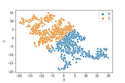
If we compare the results of our implementation and the sklearn-variant we would see that they often agree. Below the algorithms are applied to cluster two random data sets. Our implementation is to the left and the sklearn implementation is to the right.

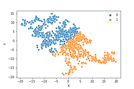
We can see that the two implementations generally agree quite well. In the top data set, they disagree on only a single point in this case: in the middle at the left most side there is a data point that our algorithm classes as cluster 0 and that the sklearn algorithm classes as cluster 1.
In the bottom data set, the two algorithms also seem to agree quite well with the clustering. The algorithms assigned different numbers to the two clusters, but the clusters themselves overlap very well between the two. In this case the two algorithms only disagree on 13 data points, out of a total of 1000 data points. Note however that for some other data sets the two might disagree more.
Comparing the speed of the two implementations we can see that while this implementation is not very much slower than the sklearn implementation, the sklearn still definately is faster.
Input: %timeit kmeans(data,k)

Output: 153 ms ± 11.2 ms per loop (mean ± std. dev. of 7 runs, 10 loops each)

Input: sklearn.clusters.k_means(data,k)

Output: 36.5 ms ± 1.03 ms per loop (mean ± std. dev. of 7 runs, 10 loops each)
This code works, but is definately not complete. The algorithm needs to be extended to handle more types of data input. For example, you might want to be able to input images. There should also be code to make sure that the parameter k is not larger than the number of data points and not less than 2.
In real-world cases you would just about never implement this algorithm yourself, but rather use one of the highly optimized libraries that exist out there, such as sklearn.
The purpose of this post was not, however, to write a complete and production-ready algorithm. Rather, the purpose of this post was to be instructive and give a better sense of the algorithm by implementing it in code.
In Conclusion
The K-Means Clustering algorithm is a solid choice amongst clustering algorithms that is even today very popular to use for data science. It is fast, simple and quite intuitive once you understand it. It is also very flexible and can be used for many many different types of data given the right pre-processing (read: given that you can somehow vectorise your data), and given that you have the right features in your data. The main weakness of K-Means is that it can be sensitive to how the centers are initialised. This is especially true if the data set is small.
I hope you enjoyed this post on how to implement the K-Means Clustering algorithm! If you liked it or have a question, please share it with a friend you think might be interested or leave a comment below! And until next time, stay ever hungry to learn!
