

Howdy fellow learner! In this post about the multi-armed bandit problem, we will start to learn about the fundamentals of reinforcement learning. To aid in our learning we will get to meet Carl and follow him as he tries to navigate the world. Along the way we will get to do some birdwatching, write some code and ponder about some philosophy. For that extra brain energy, make sure to grab a snack and a good cup of coffee before we dive in. Welcome to the learning journey, and let us begin!
This post will focus on the conceptual understanding of the multi-armed bandit problem and the algorithm used to solve it. If you already have the concept down, you should instead head over to the second part for the code implementation and analysis !
Subjects: Epsilon-Greedy Algorithm, A/B Testing, Multiple-Armed Bandit Problems, Python and a little bit of Life Philosophy thrown in for good measure. :)
Origin Story | A Bandit Is Born
The multi-armed bandit problem has it’s origins way back in 1933 when William Thompson published a paper titled “On the likelihood that one unknown probability exceeds another in view of the evidence of two samples”. Thompson studied how to think when a choice had to be made but there was too few data points to make a certain judgement. His questions and work gave rise to a field which would turn into the study of multi-armed bandit problems. More formally, a bandit problem is when we have several choices at our disposal but each choice has an unknown chance of giving a desired reward. Such a case can be a doctor trying to save as many patients as possible from a new deadly disease, without any a priori knowledge of which treatment is the most effective. Let’s call our doctor Carl.
When doing research, Dr. Carl usually create equally sized cohorts (groups) of patients and gives each cohort a different treatment. After he has the results from all the patient groups he can then determine which treatment was the best. This is all good for helping people in the future, but at the cost of the patients who got the wrong treatment. The risk is that some patients were administered the wrong treatment and potentially died needlessly. Or was it needless? Is this in fact the only approach possible, and no better solution exists? Well, not really.
Luckily for us, there are algorithms that aim to solve bandit problems by finding the best treatment while also maximising the number of patients that got the best treatment. This is called that we want to maximise the optimality of our algorithm. Another way of looking at it is that our dear doctor will have a guilty consciousness for needlessly giving the wrong treatment to patients. Thus, we want to find a strategy or algorithm that minimises the doctor’s regret. And yes, regret here actually is a technical term we’ll talk about in a future post. In this post we will primarily use the optimality way of phrasing the objective as I find it clearer to use. If you feel confused so far don’t worry – it will all clear up soon!
The term Multi-Armed Bandit comes from an old joke about the gambling machines in casinos. Each such machine had an unknown chance of giving a reward each time you pulled the lever (arm). Most of the times these machines had a single arm, and given the machine’s habit of robbing people of their money the name One-Armed Bandit was born. In life we often face several potential options to choose between each with an unknown outcome. Researchers imagined that the problem formulation of One-Armed Bandit accurately also could be extended to such problems, thinking of each choice as it’s own “arm” – thus the name Multi-Armed Bandit.
The field of solving Multi-Armed Bandit problems is part of what is known as “optimal control” in classical control theory and more recently part of “reinforcement learning” in artificial intelligence research. Algorithms for solving Multi-Armed Bandit problems have been around for a long time now, and are still actively being researched and developed. Companies such as Google and Facebook use variants of bandit algorithms to serve users the best ads, Netflix (and probably YouTube) use them to decide which content to show you and they are even used in things such deciding the optimal design of websites and which headline to have for a given article. In short, when used right they can be quite powerful.
To Explore The Unknown Or Exploit What You Know, That Is The Question | A Fundamental Question in Life
The fundamental problem at heart of all bandit problems turns out to be surprisingly deep and applicable to life in general: Should you exploit what you know is good and choose the familiar, or should you explore the unknown in hopes of finding something better?
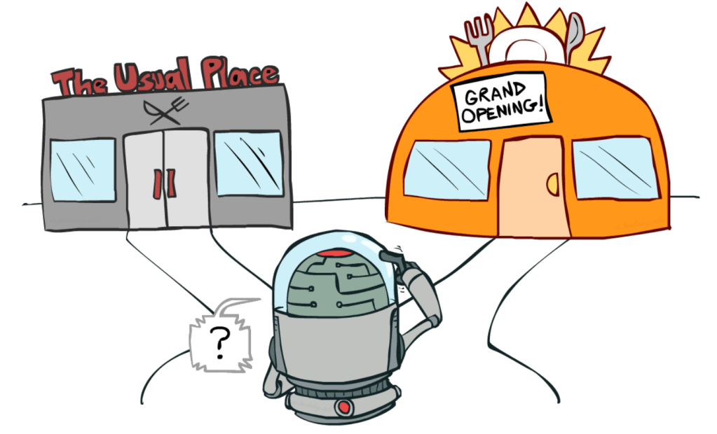
Let’s take another example of our friend Carl’s life. Carl absolutely loves eating out at his favourite diner once a week. Carl has done so consistently for the last few years and it has sort of become a cherished ritual his. One day Carl moves to a new city – Banditville – where he doesn’t know any of the restaurants except for one which is decent but not great. Ideally Carl would like to find where the best diner in the city is, but naturally he would also like to avoid having a bad eating experience. How much should he explore what diners are available in Banditville and how much should he exploit what he already knows is good. This is the famous Explore-Exploit Dilemma which lies at the core of most reinforcement learning problems.
As you begin to ponder how wide and complex the scope of this question really is, I hope you see just how useful algorithms and strategies for solving it would be! Indeed they reach far beyond the scope of machine learning and can help us make better choices in our own lives… But the explore-exploit dilemma deserves it own mini-series to be properly discussed, so let’s get back to it later on and get on with a bit more technical stuff!
The Epsilon-Greedy Bandit Algorithm | Having The Cake But Eating It Too

Full Exploration or Full Exploitation | Two Extremes
Multi-Armed Bandit problems are where you have two or more options with uncertain chances of rewards. When faced with such situations there are two extreme ways of handling them: pure exploration or pure exploitation.
A scientist or a scholar who studies the situation and wish to derive knowledge from it might be inclined to just explore all the options as much as possible before deciding which option to use. This is what is known as epsilon first (epsilon standing for exploration) or A/B testing. The common approach is usually to decide a set number of test, and then split the tests equally among each possible arm / choice. Often the number of tests is quite large and the person conducting the test is interested with being very certain about the results. A problem with this is that you risk leaving a lot of money on the table, so to speak. The reason is that during the test itself you will start to get an indication of which choice is the best one. One you get the indication that a certain choice is the best choice you increasingly risk “wasting” your resources by exploring inferior options. This can sometimes be an acceptable price in order to be scientifically rigorous – but for many real-life cases outside of academia such rigour might be overkill and the cost for rigour might not be worth it.
The other extreme to A/B testing is to simply use what you already know and exploit it 100%. This is what is known as the greedy approach. Greedy algorithms are a class of algorithms in computer science that always choose the option that seems to be the best option right now. In that sense they are quite short sighted, but has proven to be very efficient in many cases. However, in the explore-exploit dilemma any purely greedy approach has a serious flaw that becomes obvious if you think about it: The greedy approach is only possible if you know which option to choose in the first place! If that initial guess is wrong, then you will waste all your resources on the wrong bet! Worst part is – you might never even know that you settled for the inferior choice!
Epsilon-Greedy | A Golden Middle Road
Enter our algorithm to solve the dilemma; the epsilon-greedy algorithm! This algorithm is a stochastic algorithm meaning it randomly makes one of two choices:
Choice 1: Randomly choose any of the bandit’s arms to explore.
Choice 2: Choose the arm that, up until know, looks the most promising.
How often it chooses one over the other is governed by the parameter ε (read as epsilon standing for exploration). It makes a choice with probability ε, and thus with probability 1 – ε makes the currently best choice. A very common value for ε is 0.1 meaning that about 10% of the time will be based on exploring and the remaining about 90% of the time will be spent exploiting our exploration so far and selecting what we currently believe to be the best option.
Note, however, that when we say 10% chance of exploring we mean exploring all options including the option currently believed to be the best. This means that if we have two options we actually have 95% chance of choosing the best option. Let’s illustrate with a two-armed bandit with arms A and B, where we believe A is the best arm. With 90% chance we will automatically choose arm A since that is believed to be the best arm. The remaining 10% is spent on blindly exploring all options available. Since we have two arms we thus will spend half of our exploration on arm A and half of the exploration on arm B. Thus the total chance for choosing arm A is 90%+5% = 95% and the total chance for choosing arm B is 5%. If we would have ε = 0.1 and four arms A, B, C and D with A to believed to be the best we would choose A with 92.5% (90% + 10%/4).
For the sake of keeping this post brief(er), we will only go through the epsilon-greedy algorithm, even though many other algorithms exist. But going through this algorithm in detail will give us a solid feeling for the problem domain. Despite it being one of the simplest algorithms, the epsilon-greedy algorithm can often solve bandit problems with extremely high efficiency! This means that the final result of the algorithm stays very close to obtaining optimal results (defined as always choosing the right option).
Algorithmic Assumptions
Most bandit algorithms are based around the following three core assumptions:
- Each sample drawn, that is the result obtained from choosing an arm, is independent and identically distributed.
- The bandit has a single unchanging state.
- Choosing one arm yields instantaneous results.
Independent and identically distributed
The first assumption is a difficult way of saying something quite simple. It means that we assume that there is no complicated relationship between our observations and that they all behave more or less the same way. In our example above trying to cure patients, this would mean the following:
a) independent: we assume that every patient is it’s own unique person meaning we only try to cure a patient once. The same patient never returns and we never try to cure it again, regardless of results.
b) identically distributed: we assume that every patient has the same chance of being cured given a certain treatment. For example we assume no patients are horses or plants, as they likely would respond differently than humans to the treatment. Additionally, we either assume that traits such as gender, age or socio-economic status has no impact on how effective the treatment is – or we assume that if any trait has an impact then all patients have the same trait.
Single unchanging state
The second assumption is that the bandit has a single unchanging state. This assumption will make more sense as we go into more complex problems in future posts, but it basically means that the world never changes with regard to our experiment. Again drawing examples from the doctor example, such things could mean that the bacteria making our patients sick won’t evolve to suddenly become more resistant or less resistant to any of the treatment options. It also means that results gained at the start of the experiment will be just as informative as results gained at the end of the experiment with regards to the nature of the problem.
Instantaneous results
The third and final assumption basically means that we assume we can be certain that the outcome observed comes directly from the option we choose. In the doctor example that would mean that patients that die don’t die because of external effects such as being run over by a car or another unrelated cause. And people who are cured are not cured because they changed their diet or got a treatment from some other place.
In Conclusion | And Following Up With Code Implementations!
In this post we learnt about what a multi-armed bandit problem was and saw several examples of it in real life situations. We were then briefly introduced to the explore-exploit dilemma that lies at the heart of all bandit problems. Finally we discovered the epsilon-greedy algorithm and learnt more about how it works and also the fundamental assumptions lying at it’s heart. Now all that remains is putting it all in code, which we will do in the next part of this post. :)
Next Up: Bandits I: Birdwatching In Banditville|Code Implementation
And there you have it! That was it for the first episode on our learning journey towards reinforcement learning. Hope you enjoyed it and until next time, stay hungry for knowledge!
